52. Cake Eating II: Numerical Methods#
52.1. Overview#
In this lecture we continue the study of the cake eating problem.
The aim of this lecture is to solve the problem using numerical methods.
At first this might appear unnecessary, since we already obtained the optimal policy analytically.
However, the cake eating problem is too simple to be useful without modifications, and once we start modifying the problem, numerical methods become essential.
Hence it makes sense to introduce numerical methods now, and test them on this simple problem.
Since we know the analytical solution, this will allow us to assess the accuracy of alternative numerical methods.
Note
The code below aims for clarity rather than maximum efficiency.
In the lectures below we will explore best practice for speed and efficiency.
Let’s put these algorithm and code optimizations to one side for now.
We will use the following imports:
import matplotlib.pyplot as plt
import numpy as np
from scipy.optimize import minimize_scalar, bisect
from typing import NamedTuple
52.2. Reviewing the Model#
You might like to review the details before we start.
Recall in particular that the Bellman equation is
where \(u\) is the CRRA utility function.
The analytical solutions for the value function and optimal policy were found to be as follows.
def c_star(x, β, γ):

    return (1 - β ** (1/γ)) * x


def v_star(x, β, γ):

    return (1 - β**(1 / γ))**(-γ) * (x**(1-γ) / (1-γ))
Our first aim is to obtain these analytical solutions numerically.
52.3. Value Function Iteration#
The first approach we will take is value function iteration.
This is a form of successive approximation, and was discussed in our lecture on job search.
The basic idea is:
Take an arbitrary initial guess of \(v\).
Obtain an update \(w\) defined by
\[ w(x) = \max_{0\leq c \leq x} \{u(c) + \beta v(x-c)\} \]Stop if \(w\) is approximately equal to \(v\), otherwise set \(v=w\) and go back to step 2.
Let’s write this a bit more mathematically.
52.3.1. The Bellman Operator#
We introduce the Bellman operator \(T\) that takes a function v as an argument and returns a new function \(Tv\) defined by
From \(v\) we get \(Tv\), and applying \(T\) to this yields \(T^2 v := T (Tv)\) and so on.
This is called iterating with the Bellman operator from initial guess \(v\).
As we discuss in more detail in later lectures, one can use Banach’s contraction mapping theorem to prove that the sequence of functions \(T^n v\) converges to the solution to the Bellman equation.
52.3.2. Fitted Value Function Iteration#
Both consumption \(c\) and the state variable \(x\) are continuous.
This causes complications when it comes to numerical work.
For example, we need to store each function \(T^n v\) in order to compute the next iterate \(T^{n+1} v\).
But this means we have to store \(T^n v(x)\) at infinitely many \(x\), which is, in general, impossible.
To circumvent this issue we will use fitted value function iteration, as discussed previously in one of the lectures on job search.
The process looks like this:
Begin with an array of values \(\{ v_0, \ldots, v_I \}\) representing the values of some initial function \(v\) on the grid points \(\{ x_0, \ldots, x_I \}\).
Build a function \(\hat v\) on the state space \(\mathbb R_+\) by linear interpolation, based on these data points.
Obtain and record the value \(T \hat v(x_i)\) on each grid point \(x_i\) by repeatedly solving the maximization problem in the Bellman equation.
Unless some stopping condition is satisfied, set \(\{ v_0, \ldots, v_I \} = \{ T \hat v(x_0), \ldots, T \hat v(x_I) \}\) and go to step 2.
In step 2 we’ll use continuous piecewise linear interpolation.
52.3.3. Implementation#
The maximize function below is a small helper function that converts a
SciPy minimization routine into a maximization routine.
def maximize(g, a, b, args):
    """
    Maximize the function g over the interval [a, b].

    We use the fact that the maximizer of g on any interval is
    also the minimizer of -g.  The tuple args collects any extra
    arguments to g.

    Returns the maximal value and the maximizer.
    """

    objective = lambda x: -g(x, *args)
    result = minimize_scalar(objective, bounds=(a, b), method='bounded')
    maximizer, maximum = result.x, -result.fun
    return maximizer, maximum
We’ll store the parameters \(\beta\) and \(\gamma\) and the grid in a
NamedTuple called Model.
# Create model data structure
class Model(NamedTuple):
    β: float
    γ: float
    x_grid: np.ndarray

def create_cake_eating_model(β=0.96,           # discount factor
                              γ=1.5,            # degree of relative risk aversion
                              x_grid_min=1e-3,  # exclude zero for numerical stability
                              x_grid_max=2.5,   # size of cake
                              x_grid_size=120):
    """
    Creates an instance of the cake eating model.
    """
    x_grid = np.linspace(x_grid_min, x_grid_max, x_grid_size)
    return Model(β=β, γ=γ, x_grid=x_grid)
Now we define utility functions that operate on the model:
def u(c, γ):
    """
    Utility function.
    """
    if γ == 1:
        return np.log(c)
    else:
        return (c ** (1 - γ)) / (1 - γ)

def u_prime(c, γ):
    """
    First derivative of utility function.
    """
    return c ** (-γ)

def state_action_value(c, x, v_array, model):
    """
    Right hand side of the Bellman equation given x and c.
    """
    β, γ, x_grid = model.β, model.γ, model.x_grid
    v = lambda x: np.interp(x, x_grid, v_array)

    return u(c, γ) + β * v(x - c)
We now define the Bellman operation:
def T(v, model):
    """
    The Bellman operator.  Updates the guess of the value function.

    * model is an instance of Model
    * v is an array representing a guess of the value function

    """
    v_new = np.empty_like(v)

    for i, x in enumerate(model.x_grid):
        # Maximize RHS of Bellman equation at state x
        v_new[i] = maximize(state_action_value, 1e-10, x, (x, v, model))[1]

    return v_new
After defining the Bellman operator, we are ready to solve the model.
Let’s start by creating a model using the default parameterization.
model = create_cake_eating_model()
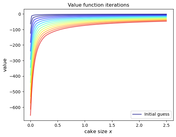
Now let’s see the iteration of the value function in action.
We start from guess \(v\) given by \(v(x) = u(x)\) for every \(x\) grid point.
x_grid = model.x_grid
v = u(x_grid, model.γ)  # Initial guess
n = 12                  # Number of iterations

fig, ax = plt.subplots()

ax.plot(x_grid, v, color=plt.cm.jet(0),
        lw=2, alpha=0.6, label='Initial guess')

for i in range(n):
    v = T(v, model)  # Apply the Bellman operator
    ax.plot(x_grid, v, color=plt.cm.jet(i / n), lw=2, alpha=0.6)

ax.legend()
ax.set_ylabel('value', fontsize=12)
ax.set_xlabel('cake size $x$', fontsize=12)
ax.set_title('Value function iterations')

plt.show()
To do this more systematically, we introduce a wrapper function called
compute_value_function that iterates until some convergence conditions are
satisfied.
def compute_value_function(model,
                           tol=1e-4,
                           max_iter=1000,
                           verbose=True,
                           print_skip=25):

    # Set up loop
    v = np.zeros(len(model.x_grid)) # Initial guess
    i = 0
    error = tol + 1

    while i < max_iter and error > tol:
        v_new = T(v, model)

        error = np.max(np.abs(v - v_new))
        i += 1

        if verbose and i % print_skip == 0:
            print(f"Error at iteration {i} is {error}.")

        v = v_new

    if error > tol:
        print("Failed to converge!")
    elif verbose:
        print(f"\nConverged in {i} iterations.")

    return v_new
Now let’s call it, noting that it takes a little while to run.
v = compute_value_function(model)
Error at iteration 25 is 23.8003755134813.
Error at iteration 50 is 8.577577195046615.
Error at iteration 75 is 3.091330659691039.
Error at iteration 100 is 1.1141054204751981.
Error at iteration 125 is 0.4015199357729671.
Error at iteration 150 is 0.14470646660561215.
Error at iteration 175 is 0.052151735472762084.
Error at iteration 200 is 0.018795314242879613.
Error at iteration 225 is 0.006773769545588948.
Error at iteration 250 is 0.0024412443051460286.
Error at iteration 275 is 0.0008798164327572522.
Error at iteration 300 is 0.00031708295392718355.
Error at iteration 325 is 0.00011427565573285392.

Converged in 329 iterations.
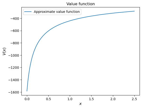
Now we can plot and see what the converged value function looks like.
fig, ax = plt.subplots()

ax.plot(x_grid, v, label='Approximate value function')
ax.set_ylabel('$V(x)$', fontsize=12)
ax.set_xlabel('$x$', fontsize=12)
ax.set_title('Value function')
ax.legend()
plt.show()
Next let’s compare it to the analytical solution.
v_analytical = v_star(model.x_grid, model.β, model.γ)
fig, ax = plt.subplots()

ax.plot(x_grid, v_analytical, label='analytical solution')
ax.plot(x_grid, v, label='numerical solution')
ax.set_ylabel('$V(x)$', fontsize=12)
ax.set_xlabel('$x$', fontsize=12)
ax.legend()
ax.set_title('Comparison between analytical and numerical value functions')
plt.show()
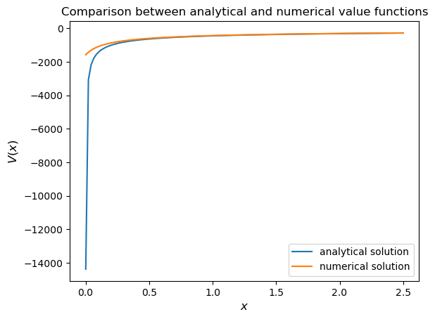
The quality of approximation is reasonably good for large \(x\), but less so near the lower boundary.
The reason is that the utility function and hence value function is very steep near the lower boundary, and hence hard to approximate.
Note
One way to fix this issue is to use a nonlinear grid, with more points in the neighborhood of zero.
Instead of pursuing this idea, however, we will turn our attention to working with policy functions.
We will see that value function iteration can be avoided by iterating on a guess of the policy function instead.
These ideas will be explored over the next few lectures.
52.3.4. Policy Function#
Let’s try computing the optimal policy.
In the first lecture on cake eating, the optimal consumption policy was shown to be
Let’s see if our numerical results lead to something similar.
Our numerical strategy will be to compute
on a grid of \(x\) points and then interpolate.
For \(v\) we will use the approximation of the value function we obtained above.
Here’s the function:
def σ(model, v):
    """
    The optimal policy function. Given the value function,
    it finds optimal consumption in each state.

    * model is an instance of Model
    * v is a value function array

    """
    c = np.empty_like(v)

    for i in range(len(model.x_grid)):
        x = model.x_grid[i]
        # Maximize RHS of Bellman equation at state x
        c[i] = maximize(state_action_value, 1e-10, x, (x, v, model))[0]

    return c
Now let’s pass the approximate value function and compute optimal consumption:
c = σ(model, v)
Let’s plot this next to the true analytical solution
c_analytical = c_star(model.x_grid, model.β, model.γ)

fig, ax = plt.subplots()

ax.plot(model.x_grid, c_analytical, label='analytical')
ax.plot(model.x_grid, c, label='numerical')
ax.set_ylabel(r'$\sigma(x)$')
ax.set_xlabel('$x$')
ax.legend()

plt.show()
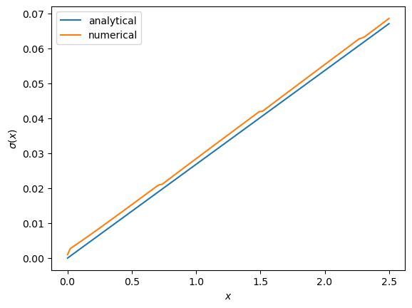
The fit is reasonable but not perfect.
We can improve it by increasing the grid size or reducing the error tolerance in the value function iteration routine.
However, both changes will lead to a longer compute time.
Another possibility is to use an alternative algorithm, which offers the possibility of faster compute time and, at the same time, more accuracy.
We explore this soon.
52.4. Exercises#
Exercise 52.1
Try the following modification of the problem.
Instead of the cake size changing according to \(x_{t+1} = x_t - c_t\), let it change according to
where \(\alpha\) is a parameter satisfying \(0 < \alpha < 1\).
(We will see this kind of update rule when we study optimal growth models.)
Make the required changes to value function iteration code and plot the value and policy functions.
Try to reuse as much code as possible.
Solution
We need to create an extended version of our model and state-action value function.
We’ll create a new NamedTuple for the extended cake model and a helper function.
# Create extended cake model data structure
class ExtendedModel(NamedTuple):
    β: float
    γ: float
    α: float
    x_grid: np.ndarray

def create_extended_model(β=0.96,           # discount factor
                          γ=1.5,            # degree of relative risk aversion
                          α=0.4,            # productivity parameter
                          x_grid_min=1e-3,  # exclude zero for numerical stability
                          x_grid_max=2.5,   # size of cake
                          x_grid_size=120):
    """
    Creates an instance of the extended cake eating model.
    """
    x_grid = np.linspace(x_grid_min, x_grid_max, x_grid_size)
    return ExtendedModel(β=β, γ=γ, α=α, x_grid=x_grid)

def extended_state_action_value(c, x, v_array, model):
    """
    Right hand side of the Bellman equation for the extended cake model given x and c.
    """
    β, γ, α, x_grid = model.β, model.γ, model.α, model.x_grid
    v = lambda x: np.interp(x, x_grid, v_array)

    return u(c, γ) + β * v((x - c)**α)
We also need a modified Bellman operator:
def T_extended(v, model):
    """
    The Bellman operator for the extended cake model.
    """
    v_new = np.empty_like(v)

    for i, x in enumerate(model.x_grid):
        # Maximize RHS of Bellman equation at state x
        v_new[i] = maximize(extended_state_action_value, 1e-10, x, (x, v, model))[1]

    return v_new
Now create the model:
model = create_extended_model()
Here’s the computed value function.
def compute_value_function_extended(model,
tol=1e-4,
max_iter=1000,
verbose=True,
print_skip=25):
"""
Compute value function for extended cake model.
"""
v = np.zeros(len(model.x_grid))
i = 0
error = tol + 1
while i < max_iter and error > tol:
v_new = T_extended(v, model)
error = np.max(np.abs(v - v_new))
i += 1
if verbose and i % print_skip == 0:
print(f"Error at iteration {i} is {error}.")
v = v_new
if error > tol:
print("Failed to converge!")
elif verbose:
print(f"\nConverged in {i} iterations.")
return v_new
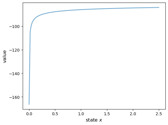
v = compute_value_function_extended(model, verbose=False)
fig, ax = plt.subplots()
ax.plot(model.x_grid, v, lw=2, alpha=0.6)
ax.set_ylabel('value', fontsize=12)
ax.set_xlabel('state $x$', fontsize=12)
plt.show()
Here’s the computed policy, combined with the solution we derived above for the standard cake eating case \(\alpha=1\).
def σ_extended(model, v):
    """
    The optimal policy function for the extended cake model.
    """
    c = np.empty_like(v)

    for i in range(len(model.x_grid)):
        x = model.x_grid[i]
        c[i] = maximize(extended_state_action_value, 1e-10, x, (x, v, model))[0]

    return c

c_new = σ_extended(model, v)

# Get the baseline model for comparison
baseline_model = create_cake_eating_model()
c_analytical = c_star(baseline_model.x_grid, baseline_model.β, baseline_model.γ)

fig, ax = plt.subplots()

ax.plot(baseline_model.x_grid, c_analytical, label=r'$\alpha=1$ solution')
ax.plot(model.x_grid, c_new, label=fr'$\alpha={model.α}$ solution')

ax.set_ylabel('consumption', fontsize=12)
ax.set_xlabel('$x$', fontsize=12)

ax.legend(fontsize=12)

plt.show()
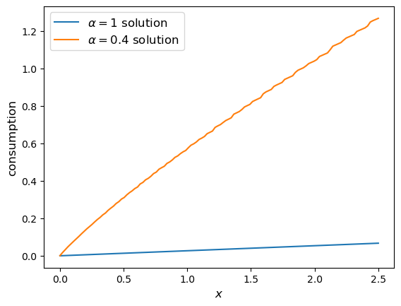
Consumption is higher when \(\alpha < 1\) because, at least for large \(x\), the return to savings is lower.